import os
import sys

import numpy as np
from astropy import units as u

import sbfit
import sbfit.model

Load data

Initialize an ObservationList object.

observations = sbfit.ObservationList()

Load images into the ObservationList object.

image_dir = "a3667/chandra"

obsids = [513, 889, 5751, 5752, 5753, 6292, 6295, 6296]

for obsid in obsids:
    observations.add_observation_from_file(f"a3667/chandra/{obsid}_band1_thresh.img",
                                           f"a3667/chandra/{obsid}_band1_thresh.expmap",
                                           f"a3667/chandra/{obsid}_band1_nxb_full.img",
                                           bkg_norm_type="count",
                                           bkg_norm_keyword="bkgnorm", )

Read region file

epanda = sbfit.read_region("a3667.reg")

Extract a profile

The region set loaded in the previous step is used.

The channel_width is the size of the radius grid for a profile. The value should be less than the psf width.

a3667_chandra_profile = observations.get_profile(epanda, channel_width=0.5)

WARNING: FITSFixedWarning: RADECSYS= 'ICRS ' / default
the RADECSYS keyword is deprecated, use RADESYSa. [astropy.wcs.wcs]
WARNING: FITSFixedWarning: 'datfix' made the change 'Set DATEREF to '1998-01-01' from MJDREF.
Set MJD-END to 51444.513808 from DATE-END'. [astropy.wcs.wcs]
WARNING: FITSFixedWarning: 'datfix' made the change 'Set DATEREF to '1998-01-01' from MJDREF.
Set MJD-END to 51797.187928 from DATE-END'. [astropy.wcs.wcs]
WARNING: FITSFixedWarning: 'datfix' made the change 'Set DATEREF to '1998-01-01' from MJDREF.
Set MJD-END to 53529.557755 from DATE-END'. [astropy.wcs.wcs]
WARNING: FITSFixedWarning: 'datfix' made the change 'Set DATEREF to '1998-01-01' from MJDREF.
Set MJD-END to 53534.009225 from DATE-END'. [astropy.wcs.wcs]
WARNING: FITSFixedWarning: 'datfix' made the change 'Set DATEREF to '1998-01-01' from MJDREF.
Set MJD-END to 53539.451968 from DATE-END'. [astropy.wcs.wcs]
WARNING: FITSFixedWarning: 'datfix' made the change 'Set DATEREF to '1998-01-01' from MJDREF.
Set MJD-END to 53532.193692 from DATE-END'. [astropy.wcs.wcs]
WARNING: FITSFixedWarning: 'datfix' made the change 'Set DATEREF to '1998-01-01' from MJDREF.
Set MJD-END to 53536.858264 from DATE-END'. [astropy.wcs.wcs]
WARNING: FITSFixedWarning: 'datfix' made the change 'Set DATEREF to '1998-01-01' from MJDREF.
Set MJD-END to 53541.426528 from DATE-END'. [astropy.wcs.wcs]

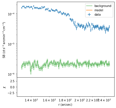
First, let’s bin the profile.

a3667_chandra_profile.rebin(130, 250,method="lin",min_cts=200,log_width=0.005,lin_width=1)
a3667_chandra_profile.plot(scale="loglog")

/Users/xyzhang/anaconda3/envs/SBFit/lib/python3.7/site-packages/sbfit-0.1.2-py3.7.egg/sbfit/profile.py:506: UserWarning: No model set.

• For Chandra observations, the PSF is small enough to use an identity smoothing matrix, which is the default setting.

• For XMM-Newton, a King profile smoothing matrix is essential to account for the broad PSF. The parameters of the profile are provided in the PSF calibration files.

a3667_chandra_profile.set_smooth_matrix("identity", king_alpha=1.4,king_rc=10,sigma=1)

Set models

Set a double power law model and load it into the profile.

The + operator can add multiple model instances into a compound model instance.

Here we use the combination of a DoublePowerLaw model and a Constant model, which represents the ICM emission and the X-ray sky background.

dpl = sbfit.model.DoublePowerLaw()
cst = sbfit.model.Constant()

a3667_chandra_profile.set_model(dpl + cst)

print(a3667_chandra_profile.model)

Model: CompoundModel
Inputs: ('x',)
Outputs: ('y',)
Model set size: 1
Expression: [0] + [1]
Components:
    [0]: <DoublePowerLaw(norm=1., a1=0.1, a2=1., r=1., c=2.)>

    [1]: <Constant(norm=0.)>
Parameters:
    norm_0 a1_0 a2_0 r_0 c_0 norm_1
    ------ ---- ---- --- --- ------
       1.0  0.1  1.0 1.0 2.0    0.0

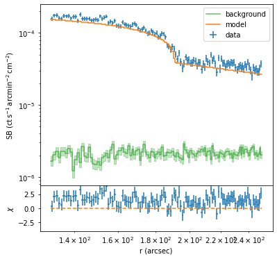
Before fit, set initial parameters that make the model profile close to the observed profile.

a3667_chandra_profile.model.norm_0 = 4e-4
a3667_chandra_profile.model.a1_0 = 0
a3667_chandra_profile.model.a2_0 = 0.6
a3667_chandra_profile.model.r_0 = 191
a3667_chandra_profile.model.c_0 = 2.4
a3667_chandra_profile.model.norm_1 = 5e-7


a3667_chandra_profile.calculate()
a3667_chandra_profile.plot()

Set parameter constraints for the model in case that the optimizer goes too far.

a3667_chandra_profile.model.norm_1.fixed = True

a3667_chandra_profile.model.norm_0.bounds = (1e-4, 6e-4)
a3667_chandra_profile.model.a1_0.bounds = (-0.7, 0.3)
a3667_chandra_profile.model.a2_0.bounds = (0.4, 1.1)
a3667_chandra_profile.model.r_0.bounds = (150, 220)
a3667_chandra_profile.model.c_0.bounds = (1.8, 3.3)

Fit

a3667_chandra_profile.fit(show_step=True, tolerance=0.01)

Start fit
C-stat: 385.679
[4.00e-04 0.00e+00 6.00e-01 1.91e+02 2.40e+00]
C-stat: 131.223
[4.06016660e-04 4.97324976e-06 5.54850695e-01 1.91013254e+02
 2.44734950e+00]
C-stat: 121.831
[4.07572762e-04 1.20461263e-04 5.54417774e-01 1.91050506e+02
 2.47224855e+00]
C-stat: 120.285
[4.06381065e-04 2.46914422e-02 5.53084590e-01 1.91106162e+02
 2.46724536e+00]
C-stat: 119.098
[4.03265749e-04 7.38250508e-02 5.47441976e-01 1.91192177e+02
 2.45016611e+00]
C-stat: 119.059
[3.98810770e-04 7.80931929e-02 5.39832122e-01 1.91245502e+02
 2.47242439e+00]
C-stat: 119.058
[3.98619753e-04 7.83445097e-02 5.39570169e-01 1.91250219e+02
 2.47354035e+00]
Iteration terminated.
Degree of freedom: 115; C-stat: 119.0578
norm_0: 3.99e-04
a1_0:   7.83e-02
a2_0:   5.40e-01
r_0:    1.91e+02
c_0:    2.47e+00
Uncertainties from rough estimation:
norm_0: 2.861e-05
a1_0:   5.164e-02
a2_0:   4.932e-02
r_0:    3.411e-01
c_0:    1.823e-01

119.0577692494737

p_bin2 = a3667_chandra_profile.deepcopy()
p_bin2.rebin(130, 250,method="lin",min_cts=200,log_width=0.005,lin_width=2)

p_bin2.fit(show_step=True)

Start fit
C-stat: 68.426
[3.98619753e-04 7.83445097e-02 5.39570169e-01 1.91250219e+02
 2.47354035e+00]
C-stat: 68.405
[3.97761118e-04 7.71829563e-02 5.38463770e-01 1.91285037e+02
 2.47927233e+00]
C-stat: 68.405
[3.97719203e-04 7.71599546e-02 5.38401152e-01 1.91286173e+02
 2.47954135e+00]
Iteration terminated.
Degree of freedom: 55; C-stat: 68.4048
norm_0: 3.98e-04
a1_0:   7.72e-02
a2_0:   5.38e-01
r_0:    1.91e+02
c_0:    2.48e+00
Uncertainties from rough estimation:
norm_0: 2.973e-05
a1_0:   5.231e-02
a2_0:   5.086e-02
r_0:    4.137e-01
c_0:    1.881e-01

68.40479742446777

The uncertainties here are obtained from the Hessian matrix in the fit routine. To better estimate the uncertainties, we need to perform a Monte-Carlo Markov Chain analysis.

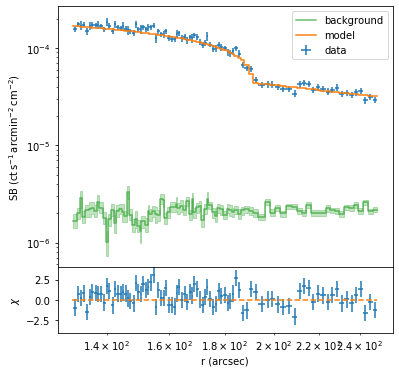
Let’s have a look of the best-fit profile first.

a3667_chandra_profile.calculate()
a3667_chandra_profile.plot(scale="loglog")

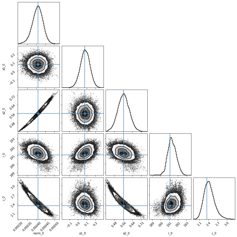
Now we use Monte-Carlo Markov Chain method to estimate the uncertainties. It takes hours to finish.

a3667_chandra_profile.mcmc_error(nsteps=5000, burnin=500)

100%|██████████| 5000/5000 [4:14:59<00:00,  3.06s/it]

norm_0: 0.0004109230243782563   +2.635e-05      -3.342e-05
a1_0:   0.07662914689543374     +6.011e-02      -5.210e-02
a2_0:   0.5632834244633022      +5.223e-02      -5.326e-02
r_0:    191.06619860779801      +7.415e-01      -3.469e-01
c_0:    2.341633374918749       +2.299e-01      -1.040e-01

The corner plot

a3667_chandra_profile.plot(plot_type="contour")

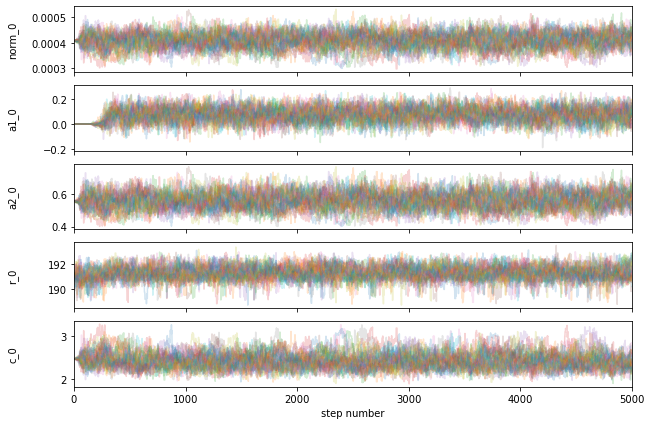
Let’s have a look how the MCMC chains walk.

a3667_chandra_profile.plot(plot_type="mcmc_chain")

The uncertainties are stored in the error attribute.

print(a3667_chandra_profile.error)

OrderedDict([('norm_0', (-0.0001161550959459374, 0.00017582104069271547)), ('a1_0', (0.1246562346145155, -0.012366244840581183)), ('a2_0', (-0.21978370273262526, 0.3234329256974142)), ('r_0', (2.2220377039538732, -1.2221756410102955)), ('c_0', (0.7662772913197773, -0.4141295370661364))])

a3667_chandra_profile.calculate()

/Users/xyzhang/anaconda3/envs/my/lib/python3.7/site-packages/sbfit-0.1.2-py3.7.egg/sbfit/profile.py:354: RuntimeWarning: invalid value encountered in true_divide
/Users/xyzhang/anaconda3/envs/my/lib/python3.7/site-packages/sbfit-0.1.2-py3.7.egg/sbfit/statistics.py:31: RuntimeWarning: invalid value encountered in true_divide

111.03038901613105